Coherence Bandwidth of Rice Channels for Millimeter Wave and Sub-Terahertz Applications

Werner Mohr

Technical University of Belin, Germany
E-mail: werner.mohr@campus.tu-berlin.de
Manuscript received 28 July 2023, accepted 23 November 2023, and ready for publication 21 March 2024.
© 2024 River Publishers

Abstract

6G research in the millimeter wave and sub-Terahertz domain is targeting very wideband systems with significantly higher data throughput than for 5G systems. Multipath propagation under shadowing conditions is affecting radio propagation, where multipath propagation results in frequency-selective fading, which is characterized by the coherence bandwidth and the time variation by the coherence time. In these frequency ranges shadowing can be overcome by additional means in the network deployment such as reflectors, RIS arrays or repeaters, which provide at the receiver a channel impulse response with a strong component (Rice type channel). Coherence bandwidth and coherence time are well-known for Rayleigh channels. However, both parameters for Rice channels versus the Rice factor $K^{'}$ are not available. This paper is investigating the coherence bandwidth and time for Rice channels based on an approximative approach for the fading statistics. With the proposed correlation criterion, the coherence bandwidth and time tend to infinity from a Rice factor around $K^{'} \geq 4 \hat{=} 6$ dB. These relations are provided by approximative functions for $K^{'} \geq 0$ starting at the Rayleigh channel.

Keywords: Coherence bandwidth, coherence time, Rayleigh channel, rice channel.

1 Introduction

6G (sixth generation of mobile communication) is targeting high aggregated carrier throughput rates in the order of several hundred Gbit/s or up to a Terabit/s (e.g., [1]), which requires very wideband radio channels. Such wide carrier bandwidth will only be available in the millimeter wave or sub-Terahertz domain. Pathloss in these frequency ranges is very high, because additional effects of atmospheric, rain and foliage attenuation need to be considered. Radio propagation is interrupted by obstacles or shadowing ([2] to [5]). In addition, multipath propagation needs to be considered, where the amplitude statistics of the received signal can be described in cases without a strong component in the channel impulse response by a Rayleigh distribution or in cases with a strong component by a Rice distribution ([5] to [7]).

Under shadowing conditions, usually a Rayleigh channel can be expected. If by additional technical means like reflectors, RIS arrays (Reconfigurable Intelligent Surfaces) or repeaters a strong component in the channel impulse response is created to shape the radio channel [8] in order to increase the received power compared to the Rayleigh channel, the channel can be characterized by a Rice channel.

Multipath propagation results in frequency-selective fading, where for certain frequencies in the channel transfer function deep fades may occur. The frequency-selectivity is characterized by the channel coherence bandwidth. For very wideband systems and delays in the channel impulse response, which are significantly bigger than the signal symbol duration, a huge channel equalization effort at the receiver is required. Therefore, a big coherence bandwidth is desired.

This paper is investigating the coherence bandwidth of Rice channels and especially its relation to the Rice factor $K^{'}$ to increase the coherence bandwidth compared to a Rayleigh channel under similar propagation conditions but without additional technical means (reflectors, RIS or repeaters).

Section 2 is describing the interference scenario and the signal model, Section 3 provides the approach to calculate the channel coherence bandwidth with the envelope correlation function and Section 4 is calculating/estimating the coherence bandwidth and coherence time of Rayleigh and Rice channels. Results are summarized in Section 5.

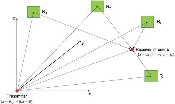
2 Interference Scenario and Signal Model

2.1 Channel Impulse Response for Multipath Propagation

The multipath propagation scenario between the transmitter and receiver of user $k$ is shown in Figure 1. The different $I$ multipath components may be caused by reflecting areas $R_{1}$ to $R_{I}$ like walls, metallic reflectors, RIS arrays or repeaters. In general, there is also a direct component between transmitter and receiver or a strong component under shadowing conditions, which is enforced by metallic reflectors, RIS arrays or repeaters [8]. The channel impulse response follows in (1).

h_{m p} (t) = h_{s} \cdot δ (t) + \sum_{i = 1}^{I} h_{r, i} \cdot δ (t - τ_{i})

(1)

Figure 1 General multipath propagation scenario between transmitter and receiver of user $k$ .

In the following it is assumed that the direct or strong component $h_{s}$ occurs at the beginning of the channel impulse response at relative delay $τ = 0$ . If a RIS is applied as a reflecting area, each multipath component $h_{r, i}$ comprises $M \cdot N$ sub-components from the reflection of each RIS element, which may add a slightly different delay $Δ τ_{R I S, i, m, n, k}$ . In the following it is assumed that all involved RIS arrays may have the same size $M \cdot N$ . It is assumed that the different RIS elements are electromagnetically mutually independent from each other for a spacing $\geq λ / 2$ ( $λ$ wavelength) like for antenna arrays [9], pp. 254.

Figure 2 is describing the propagation scenario for a RIS array $R_{i}$ . The reflection coefficient or Radar cross section $ϱ {(material, ϕ_{i}, ϕ_{r})}_{i, m, n, k}$ of each RIS element is changing – depending on the material – the amplitude and angle $ϕ_{r}$ of the reflected wave in relation to the amplitude and angle $ϕ_{i}$ of the incoming wave. A RIS array shows some beamforming capabilities to direct the outgoing wave to a specific direction.

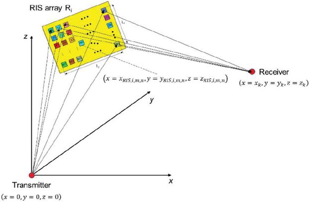
Figure 2 Propagation scenario for RIS array $R_{i}$ between transmitter and receiver of user $k$ .

The sum of all contributions $h_{t r, i, k} (t)$ via a RIS array $R_{i}$ is given in (2.1) with the contributions $h_{t R, i, m, n}$ and delay $τ_{t R, i, m, n}$ from the transmitter to RIS element $i, m, n$ and $h_{R r, i, m, n, k}$ and delay $τ_{R r, i, m, n, k}$ from the RIS element $i, m, n$ to the receiver of user $k$ and a RIS element internal delay $Δ τ_{i, m, n, k}$ .

$h_{t r, i, k} (t)$	$= \sum_{m = 1}^{M} \sum_{n = 1}^{N} {h_{t R, i, m, n} \cdot ϱ {(material, ϕ_{i}, ϕ_{r})}_{i, m, n, k}$
	$\cdot h_{R r, i, m, n, k} \cdot δ (t - τ_{t R, i, m, n} - Δ τ_{i, m, n, k} - τ_{R r, i, m, n, k})}$
	$\approx h_{r, i} \cdot δ (t - τ_{i})$	(2)

Due to the rather small physical RIS size compared to the distance between transmitter and receiver the delay differences between the different RIS elements do not result in a significant frequency dependency. The RIS elements can be used for beam steering towards a specific direction.

However, the entire impulse response $h_{t r, k} (t)$ between transmitter and receiver of user $k$ follows as the sum of all $I$ multipath components plus the direct component in (2.1).

$h_{t r, k} (t)$	$= h_{s, k} \cdot δ (t) + \sum_{i = 1}^{I} \sum_{m = 1}^{M} \sum_{n = 1}^{N} {h_{t R, i, m, n}$
	$\cdot ϱ {(material, ϕ_{i}, ϕ_{r})}_{i, m, n, k} \cdot h_{R r, i, m, n, k}$
	$\cdot δ (t - τ_{t R, i, m, n} - Δ τ_{i, m, n, k} - τ_{R r, i, m, n, k})}$
	$\approx h_{s} \cdot δ (t) + \sum_{i = 1}^{I} h_{r, i} \cdot δ (t - τ_{i})$	(3)

In general, the bigger delay differences between the different $I$ multipath components remain, which are responsible for the frequency dependency of the RIS transmission [10] which is sensitive to the user location.

If beam steering in the RIS system by appropriate outgoing angles of reflected waves is applied, a strong multipath component towards user $k$ may be created by avoiding additional strong components, which is reducing the frequency dependency. However, these reflected waves in other directions may cause interference or strong frequency dependency for other users.

2.2 Signal Model to Derive the Coherence Bandwidth of the Rice Channel

The applied signal model for the Rice channel is based on [11], pp. 45. In the following the channel impulse response with a dominant component is described by (1). If the number of arriving partial waves $I \to \infty$ , (1) is replaced by (4).

h_{R i c e, m p} (t) = h_{s} \cdot δ (t) + h (t)

(4)

$h_{s} \cdot δ (t)$ corresponds to the dominant component and $h (t)$ describes the scattering part from many different sources.

With the notation in [11], pp. 13 the transmitted signal is described in (5) with the E-field component in z-direction.

s_{t} (t) = E_{z, 0} \cdot \cos (ω_{0} \cdot t)

(5)

The received signal $s_{r} (t)$ is affected by Doppler shift $ω_{d, j}$ versus different angles of arrival $ϑ_{j}$ and wavelength $λ$ or frequency $f$ , speed of light $c_{0}$ and mobile speed $υ$ [11], p. 20.

$β = \frac{2 π}{λ} = \frac{2 π \cdot f}{c_{0}} = \frac{ω}{c_{0}}$
$ω_{d, j} = \frac{2 π}{λ} \cdot υ \cdot \cos ϑ_{j}$	(6)

At each Doppler shift $ω_{d, j}$ corresponding to $\pm ϑ_{j}$ signals with different delay $τ_{j, i}$ may occur or at each delay $τ_{j, i}$ partial waves with different Doppler shift $ω_{d, j}$ are received.

With these considerations the received signal is described as the sum of all different wave components versus Doppler shift $ω_{d, 0}$ of the dominant component and versus delay $τ_{j, i}$ and Doppler shift $ω_{d, j}$ for the scattering part with the amplitude coefficients $C_{0, 0}$ and $C_{j, i}$ with $I$ and $J \to \infty$ .

$E_{z} (ω, t)$	$= E_{z, 0} \cdot C_{0, 0} \cdot \cos (ω \cdot t + ω_{d, 0} \cdot t)$
	$+ E_{z, 0} \cdot \sum_{j = 1}^{J} \sum_{i = 1}^{I} C_{j, i} \cdot \cos (ω \cdot t + ω_{d, j} \cdot t - ω \cdot τ_{j, i})$	(7)

The amplitude coefficients are defined via the square root of the received power normalized to the transmitted power, which corresponds to the pathloss. With the receiver antenna azimuth diagram $G (ϑ)$ and the received power $P (ϑ_{0}, τ_{s})$ of the dominant component and the fraction of received power $p (ϑ_{j}, τ_{j, i})$ within $d ϑ d τ$ for the scattered part the coefficients $C_{0, 0}$ and $C_{j, i}$ can also be interpreted as the amplitudes of the channel impulse response of the partial waves (8). The sum of all partial waves with the same delay but different angle of arrival or Doppler shift is given in (9), which is related to (1) and (4).

$\frac{C_{0, 0}}{\sqrt{G (ϑ_{0})}}$	$= \sqrt{P (ϑ_{0}, τ_{s})} = \| h_{s} \|$
$\frac{C_{j, i}}{\sqrt{G (ϑ_{j})}}$	$= \sqrt{p (ϑ_{j}, τ_{j, i}) d ϑ d τ} = \| h_{j, i} \|$	(8)
$h_{r, i} (τ_{i})$	$= \sum_{j = 1}^{J} h_{j, i} (τ_{i})$	(9)

For simplification it is assumed that the phase angles in (2.2) are related to the phase angle of the dominant component. Then $E_{z} (ω, t)$ in (2.2) is replaced by $E_{z}^{'} (ω, t)$ in (10) and can be represented with [12], p. 156 by in-phase $x_{1} (t)$ and quadrature components $x_{2} (t)$ in (11).

$E_{z}^{'} (ω, t)$	$= E_{z, 0} \cdot C_{0, 0} \cdot \cos (ω \cdot t) + E_{z, 0} \cdot \sum_{j = 1}^{J} \sum_{i = 1}^{I} C_{j, i}$
	$\cdot \cos (ω \cdot t + (ω_{d, j} - ω_{d, 0}) \cdot t - ω \cdot τ_{j, i})$	(10)
$E_{z}^{'} (ω, t)$	$= E_{z, 0} \cdot C_{0, 0} \cdot \cos (ω \cdot t) + E_{z, 0} \cdot \sum_{j = 1}^{J} \sum_{i = 1}^{I} C_{j, i} \cdot {\cos (ω \cdot t)$
	$\cdot \cos ((ω_{d, j} - ω_{d, 0}) \cdot t - ω \cdot τ_{j, i}) - \sin (ω \cdot t)$
	$\cdot \sin ((ω_{d, j} - ω_{d, 0}) \cdot t - ω \cdot τ_{j, i})}$
	$= x_{1} (t) \cdot \cos (ω \cdot t) - x_{2} (t) \cdot \sin (ω \cdot t)$	(11)

With the assumptions in [11], pp. 47 on the stationarity of the parameters and $E_{z}^{'} (ω, t)$ corresponds to a random process, where the phase angles $ψ_{j, i}$ of sample functions of the individual waves are uniformly distributed random independent variables with $0 \leq ψ_{j, i} \leq 2 π$ , $E_{z}^{'} (ω, t)$ is regarded as a wide-sense stationary process with respect to ensemble averages. However, it is not stationary with respect to time averages, because over time and distance time delays and angles of arrivals are slowly changing. Therefore, the process is not strictly ergodic. With an increasing number of waves – which is assumed here – the difference between ensemble and time averages decreases. Therefore, in the following ensemble averages are used for the calculation.

The definition of a specific model for the channel impulse response and propagation conditions follows the same assumptions as in [11], pp. 46. For simplification it is assumed that at the receiver location partial waves arrive from all directions with a uniform distribution.

p (ϑ) = \frac{1}{2 π}

(12)

From practical experience the shape of the density of the square of the channel impulse response versus delay $τ$ (power delay profile) based on many scatterers without a dominant component corresponds to an exponential function and is interpreted as a probability distribution function $p (τ)$ of the received power versus delay normalized to the transmitted power.

p (τ) = \frac{1}{s} \cdot e^{- τ / s} with \int_{0}^{\infty} \frac{1}{s} \cdot e^{- τ / s} d τ = 1

(13)

The parameter $s$ in (13) directly corresponds to the delay spread [4], pp. 160 of the scattering part of the channel impulse response without the direct component. Both probability distribution functions are assumed to be statistically independent. Therefore, it follows [11], p. 50:

p (ϑ, τ) = \frac{1}{2 π} \cdot \frac{1}{s} \cdot e^{- τ / s}

(14)

The direct component in the Rice channel has the probability distribution in (15).

p_{s} (ϑ, τ) = δ (ϑ - ϑ_{0}) \cdot δ (τ)

(15)

With (8) this is related to the channel impulse response.

$P (ϑ_{0}, τ = 0)$	$= \frac{C_{0, 0}^{2}}{G (ϑ_{0})} \cdot p_{s} (ϑ, τ) = {\| h_{s} \|}^{2} \cdot δ (ϑ - ϑ_{0}) \cdot δ (τ)$
$p (ϑ, τ)$	$= \frac{C {(ϑ, τ)}^{2}}{G (ϑ)} = {\| h (ϑ, τ) \|}^{2} = \frac{1}{2 π} \cdot \frac{1}{s} \cdot e^{- τ / s}$	(16)

In the following the amplitude of the transmitted E-field signal is set to (17) and for the mobile station an omni-directional antenna is assumed in (18).

$E_{z, 0} = 1$	(17)
$G (ϑ) = 1$	(18)

3 Approach for Coherence Bandwidth Calculation with Envelope Correlation Function

The frequency and time dependency of the radio channel in (11) can be characterized by the coherence bandwidth $B_{c}$ and coherence time $Δ t_{c},$ which depend on the correlation between the signal envelopes at different frequencies $ω_{1}$ and $ω_{2}$ (frequency shift $Δ ω = ω_{2} - ω_{1}$ ) and time instants $t_{1}$ and $t_{2}$ (time shift $Δ t = t_{2} - t_{1}$ ). The Doppler shift at $ω_{1}$ and $ω_{2}$ is basically the same for only slightly different carrier frequencies (small relative coherence bandwidth). However, the phase at different time instants is different. The detailed mathematical calculation is provided in Annex 1.

Annex 1.A shows the detailed description of the in-phase and quadrature components $x_{1} (t)$ , $x_{2} (t)$ , $x_{3} (t)$ and $x_{4} (t)$ at $ω_{1}$ and $ω_{2}$ and also their representation by amplitude (envelope) $r$ and phase $θ$ in polar coordinates (Figure 3).

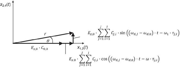
Figure 3 Representation of (A3) to (A6) by amplitude $r$ and phase $θ$ in polar coordinates from the in-phase and quadrature components $x_{1} (t)$ and $x_{2} (t)$ or $x_{3} (t)$ and $x_{4} (t)$ , respectively.

The envelope cross-correlation function $R_{e}$ between the envelopes in (A9) follows from the ensemble average of $r_{1}$ and $r_{2}$ by means of the joint probability distribution $p (r_{1}, r_{2})$ in (Annex 1.B). $p (r_{1}, r_{2})$ is derived in Annex 1.C in (A19) from the joint probability distribution $p (x_{1}, x_{2}, x_{3}, x_{4})$ in (A16) of the quadrature components by variable substitution to polar coordinates $r$ and $θ$ (Figure 3).

4 Coherence Bandwidth of Radio Channels

4.1 Coherence Bandwidth of the Rayleigh Channel

The coherence bandwidth for the Rayleigh channel can analytically be calculated by means of the complete Elliptic integral $E (k)$ of the second kind. The basic complex calculation is shown in [11], pp. 45, however, without several intermediate steps.

The envelope cross-correlation function $R_{e} (Δ ω, Δ t)$ follows with [11], p. 51 and $λ$ according to (A15) in (19).

R_{e} (Δ ω, Δ t) = μ ϵ \cdot (1 + λ) \cdot E (\frac{2 \cdot \sqrt{λ}}{1 + λ})

(19)

In [11], p. 51 the coherence bandwidth $B_{c}$ and time $Δ t_{c}$ is defined by the correlation coefficient $ϱ_{e, C o v} (Δ ω, Δ t)$ or covariance (CoV) between the two Rayleigh distributed envelopes $r_{1}$ and $r_{2}$ , which are separated versus frequency $Δ ω$ or time $Δ t$ , as defined in [15], p. 108 and 150. The correlation between both envelopes can also be expressed by the normalized cross-correlation function (CCF) $ϱ_{e, CCF} (Δ ω, Δ t)$ , which will be relevant for the Rice channel.


$ϱ_{e, C o v} (Δ ω, Δ t)$	$= \frac{⟨ r_{1} \cdot r_{2} ⟩ - ⟨ r_{1} ⟩ \cdot ⟨ r_{2} ⟩}{\sqrt{(⟨ r_{1}^{2} ⟩ - {⟨ r_{1} ⟩}^{2}) \cdot (⟨ r_{2}^{2} ⟩ - {⟨ r_{2} ⟩}^{2})}}$	(20a)
$ϱ_{e, CCF} (Δ ω, Δ t)$	$= \frac{⟨ r_{1} \cdot r_{2} ⟩}{\sqrt{⟨ r_{1}^{2} ⟩ \cdot ⟨ r_{2}^{2} ⟩}}$	(20b)

The covariance in (20a) is characterizing the fluctuation around the mean of the process, where the normalized cross-correlation function in (20b) ([15], pp. 215) is characterizing the fluctuation of the entire random process including the mean value.

With the different elements in (20a) and (20b) and the variance $σ^{2} = μ$ of the Gaussian processes $x_{1}$ , $x_{2}$ , $x_{3}$ and $x_{4}$ in (21a) to (21d) $ϱ_{e, C o v} (Δ ω, Δ t)$ and $ϱ_{e, CCF} (Δ ω, Δ t)$ result in (22) and (23).

$⟨ r_{1} \cdot r_{2} ⟩ = R_{e} (Δ ω, Δ t)$	$(19)$	(21a)
$⟨ r_{1} ⟩ = ⟨ r_{2} ⟩ = \sqrt{\frac{π}{2}} \cdot σ$	[6], p. 65	(21b)
$⟨ r_{1}^{2} ⟩ = ⟨ r_{2}^{2} ⟩ = 2 \cdot σ^{2}$	[6], p. 65	(21c)
$μ = ⟨ x_{1}^{2} ⟩ = σ^{2}$	[6], p. 64 and (A13)	(21d)
$ϱ_{e, C o v} (Δ ω, Δ t)$	$= \frac{(1 + λ) \cdot E (\frac{2 \cdot \sqrt{λ}}{1 + λ}) - \frac{π}{2}}{2 - \frac{π}{2}}$	(22)
$ϱ_{e, CCF} (Δ ω, Δ t)$	$= \frac{(1 + λ) \cdot E (\frac{2 \cdot \sqrt{λ}}{1 + λ})}{2}$	(23)

In [11], p. 51 the coherence bandwidth $B_{c}$ is defined for $ϱ_{e, C o v} (Δ ω, Δ t) = 0.5$ . From the numerical evaluation of (22) this condition is achieved at $λ_{c} = 0.725$ with (A15) and the approximation in (24) for practical applications [11], p. 51. For $λ_{c} = 0.725$ the normalized cross correlation function $ϱ_{e, CCF} (Δ ω, Δ t) = 0.893$ .

λ_{c}^{2} = \frac{J_{0}^{2} (ω \cdot \frac{υ}{c_{0}} \cdot Δ t)}{1 + s^{2} \cdot Δ ω^{2}} = {0.725}^{2} = 0.53 \approx 0.5

(24)

(25) and (26) provide the coherence bandwidth $B_{c}$ for mobile speed $υ = 0$ and/or time shift $Δ t = 0$ and the coherence time $Δ t_{c}$ as a function of maximum Doppler shift $f_{m}$ for $Δ ω = 0$ [4], p. 165.

$B_{c}$	$\approx \frac{Δ ω}{2 \cdot π} = \frac{1}{2 \cdot π \cdot s}$	(25)
$\sqrt{\frac{1}{2}}$	$\approx J_{0} (ω \cdot \frac{υ}{c_{0}} \cdot Δ t) Δ t_{c} \approx 1.13 \cdot \frac{1}{2 \cdot π \cdot f_{m}} = \frac{9}{16 \cdot π} \cdot \frac{1}{f_{m}}$	(26)

The covariance in (22) and the normalized cross-correlation function in (23) for the correct solution by means of the complete Elliptic integral is shown in Figures 4 and 5.

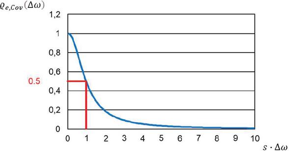
Figure 4 Covariance for the Rayleigh channel versus frequency shift $s \cdot Δ ω$ from (22).

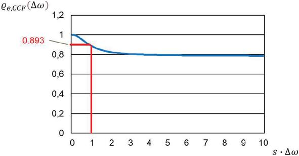
Figure 5 Normalized cross-correlation for the Rayleigh channel versus frequency shift $s \cdot Δ ω$ from (23).

The relation between covariance $ϱ_{e, C o v} (Δ ω, Δ t) = 0.5$ corresponding to the normalized cross-correlation $ϱ_{e, CCF} (Δ ω, Δ t) = 0.893$ will be applied to the Rice channel.

4.2 Coherence Bandwidth of the Rice Channel

The method in Section 4.1 with an analytical solution cannot directly be applied to the Rice channel, because the joint probability density function in (A18) is very complex for $| h_{s} | > 0$ . Therefore, an approximative approach is used for the Rice factor $K^{'} ≫ 1$ for the Rice distribution in Annex 2.A and the derivation of the envelope cross-correlation function in Annex 2.B. $K^{'}$ is defined in (27) [5], pp. 134 and $σ^{2} = μ$ in (A13). With the condition (17) the amplitude of the strong component $r_{s}$ is replaced by $r_{s} = | h_{s} |$ .

K^{'} = \frac{r_{s}^{2}}{2 \cdot σ^{2}} = \frac{{| h_{s} |}^{2}}{2 \cdot σ^{2}}

(27)

The comparison in Figure 6 between the normalized Rice distribution in (A20) and the normalized Gaussian distribution in (A25) as approximation versus the Rice factor $K^{'}$ shows a good similarity for $K^{'} > 2$ but deviations for $K^{'} < 2$ .

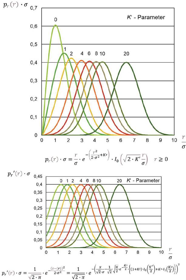
Figure 6 Upper Figure: Normalized Rice distribution $p_{r} (r) \cdot σ$ according to (A20) versus $K^{'}$ . Lower Figure: Normalized Gaussian approximation $p_{r}^{'} (r) \cdot σ$ according to (A25) versus $K^{'}$ with the mean of the Rice distribution in (A21).

The covariance $ϱ_{e, C o v} (Δ ω, Δ t)$ and the normalized cross-correlation function $ϱ_{e, CCF} (Δ ω, Δ t)$ follow directly from (20) versus $K^{'}$ , which are provided for the coherence bandwidth and coherence time.

$ϱ_{e, C o v} (Δ ω, Δ t)$	$= \frac{⟨ r_{1} \cdot r_{2} ⟩ - ⟨ r_{1} ⟩ \cdot ⟨ r_{2} ⟩}{\sqrt{(⟨ r_{1}^{2} ⟩ - {⟨ r_{1} ⟩}^{2}) \cdot (⟨ r_{2}^{2} ⟩ - {⟨ r_{2} ⟩}^{2})}}$
	$= \frac{{⟨ r ⟩}^{2} + μ_{1}^{'} - ⟨ r ⟩ \cdot ⟨ r ⟩}{\sqrt{(⟨ r^{2} ⟩ - {⟨ r ⟩}^{2}) \cdot (⟨ r^{2} ⟩ - {⟨ r ⟩}^{2})}}$
	$= \frac{μ_{1}^{'}}{⟨ r^{2} ⟩ - {⟨ r ⟩}^{2}} = \frac{μ_{1}^{'}}{σ^{2}}$	(28)
$ϱ_{e, CCF} (Δ ω, Δ t)$	$= \frac{⟨ r_{1} \cdot r_{2} ⟩}{\sqrt{⟨ r_{1}^{2} ⟩ \cdot ⟨ r_{2}^{2} ⟩}}$
	$= \frac{{⟨ r ⟩}^{2} + μ_{1}^{'}}{⟨ r^{2} ⟩} = \frac{{⟨ r ⟩}^{2} + μ_{1}^{'}}{σ^{2} + {⟨ r ⟩}^{2}} = \frac{{⟨ r ⟩}^{2} + μ_{1}^{'}}{μ^{'}}$	(29)

The covariance $ϱ_{e, C o v} (Δ ω, Δ t)$ is independent of the Rice factor $K^{'}$ (corresponding to [24]), where the normalized cross-correlation function depends on $K^{'}$ . However, with increasing $K^{'}$ the different representations of the random processes $r_{1}$ and $r_{2}$ are increasingly similar and for $K^{'} \to \infty$ both are the same, i.e., the correlation between $r_{1}$ and $r_{2}$ tends to 1. Therefore, for the Rice channel with a strong component the normalized cross-correlation function in (29) is a reasonable measure to derive the coherence bandwidth.

Coherence bandwidth $Δ ω = 2 π B_{c}$ : In this case the mobile speed is assumed $υ = 0$ . Then, the angle of arrival $ϑ_{0}$ of the strong component does not matter. With (28) $ϱ_{e, C o v} (Δ ω)$ with the delay spread $s$ of the channel impulse response without the strong component is provided in (30). Figure 7 is comparing (30) as the Rice approximation with the correct formula for the Rayleigh channel in (22) and the Rayleigh approximation in (24). There is nearly no difference between the different representations.

ϱ_{e, C o v} (Δ ω) = \frac{1}{1 + s^{2} \cdot Δ ω^{2}}

(30)

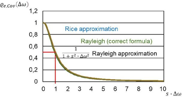
Figure 7 Coherence bandwidth $2 π B_{c}$ based on the covariance of the cross-correlation function, comparison of (30) with (22) and (24).

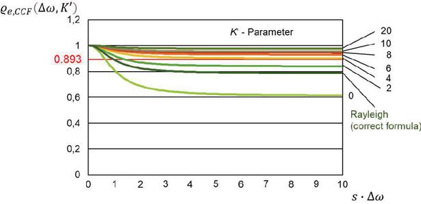
Figure 8 Coherence bandwidth $2 π B_{c}$ based on the normalized cross-correlation function with the mean according to (A21), $K^{'}$ from 0 to 20, comparison of (31) with (20b) and (23).

The normalized cross-correlation function $ϱ_{e, CCF} (Δ ω, K^{'})$ with (29) and $⟨ r (K^{'}) ⟩$ in (A21) as a function of $K^{'}$ is given in (31). Figure 8 is showing the evaluation of (31) and comparing it with (20b) and for the Rayleigh channel in (23). As can be expected from the comparison of the Rice distribution and the Gaussian approximation in Figure 6, the Gaussian approximation for $ϱ_{e, CCF} (Δ ω, K^{'})$ leads to a too low correlation for $K^{'} < 2$ . For $K^{'} > 2$ the correlation $ϱ_{e, CCF} (Δ ω, K^{'})$ provides a good approximation.

ϱ_{e, CCF} (Δ ω, K^{'}) = \frac{\frac{{⟨ r ⟩}^{2}}{σ^{2}} + \frac{1}{1 + s^{2} \cdot Δ ω^{2}}}{1 + \frac{{⟨ r ⟩}^{2}}{σ^{2}}}

(31)

With the condition $ϱ_{e, CCF} (Δ ω, K^{'}) = 0.893$ applied to (31) as for the Rayleigh channel the coherence bandwidth can be calculated from numerical evaluation, which provides a too small coherence bandwidth for $K^{'} < 2$ . With $Δ ω \cdot s \approx 1$ in (24) for the Rayleigh channel an approximative formula is derived, which is valid in the entire range $K^{'} \geq 0$ (32). From $K^{'} \geq 3.63$ the coherence bandwidth $2 π B_{c} \cdot s \to \infty$ with the definition above. Figure 9 shows the good fit of (32) for the entire range including the limiting case of the Rayleigh channel at $K^{'} = 0$ .

s \cdot 2 π B_{c} \approx {(\frac{3.63}{3.63 - K^{'}})}^{0.5250} 0 \leq K^{'} \leq 3.63

(32)

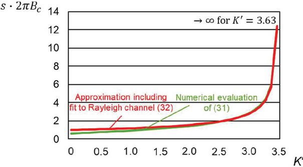
Figure 9 Normalized coherence bandwidth versus $K^{'}$ based on (31) and the approximation in (32).

Coherence time $Δ t_{c}$ : In this case the frequency shift is assumed $Δ ω = 0$ as well as the angle of arrival $ϑ_{0} = 0$ of the strong component. With (28) $ϱ_{e, C o v} (Δ t)$ with the delay spread $s$ of the channel impulse response without the strong component is provided in (33). This differs for bigger time shifts from (24) from the Rayleigh channel.

ϱ_{e, C o v} (Δ t) = J_{0} (ω \cdot \frac{υ}{c_{0}} \cdot Δ t) \cdot \cos (ω \cdot \frac{υ}{c_{0}} \cdot Δ t)

(33)

The normalized cross-correlation function $ϱ_{e, CCF} (Δ t, K^{'})$ with (29) and $⟨ r (K^{'}) ⟩$ in (A21) as a function of $K^{'}$ is given in (4.2). As can be expected from the comparison of the Rice distribution and the Gaussian approximation in Figure 6, the Gaussian approximation for $ϱ_{e, CCF} (Δ t, K^{'})$ leads to a too low correlation for $K^{'} < 2$ . For $K^{'} > 2$ the correlation $ϱ_{e, CCF} (Δ ω, K^{'})$ provides a good approximation.

ϱ_{e, CCF} (Δ t, K^{'}) = \frac{\frac{{⟨ r ⟩}^{2}}{σ^{2}} + J_{0} (ω \cdot \frac{υ}{c_{0}} \cdot Δ t) \cdot \cos (ω \cdot \frac{υ}{c_{0}} \cdot Δ t)}{1 + \frac{{⟨ r ⟩}^{2}}{σ^{2}}}

With the condition $ϱ_{e, CCF} (Δ t, K^{'}) = 0.893$ applied to (4.2) as for the Rayleigh channel the coherence time can be calculated from numerical evaluation, which provides a too small coherence time for $K^{'} < 2$ . With $ω \cdot \frac{υ}{c_{0}} \cdot Δ t_{c} \approx 1.13$ in (26) for the Rayleigh channel an approximative formula is derived, which is valid in the entire range $K^{'} \geq 0$ (4.2). From $K^{'} \geq 4.075$ the coherence time $ω \cdot \frac{υ}{c_{0}} \cdot Δ t_{c} \to \infty$ with the definition above.

ω \cdot \frac{υ}{c_{0}} \cdot Δ t_{c} \approx 1.13 \cdot {(\frac{4.075}{4.075 - K^{'}})}^{0.117} 0 \leq K^{'} \leq 4.075

4.3 Relation Between the Delay Spread of the Rayleigh and the Rice Channel

With the definition of the delay spread in [4], pp. 160 a relation between the delay spread between the Rayleigh and the Rice channel can be derived in (36) under the assumption that the strong component in the Rice channel occurs at the beginning of the channel impulse response at $τ = 0$ . With increasing $K^{'}$ $s_{Rice}$ is decreasing for constant $s_{Rayleigh}$ .

{s_{Rice} |}_{τ = 0} = s_{Rayleigh} \cdot \sqrt{\frac{1}{K^{'} + 1} \cdot (2 - \frac{1}{K^{'} + 1})}

(36)

4.4 Practical Applications

Especially in the millimeter wave and sub-Terahertz domain coverage under shadowing conditions can only be ensured by additional technical means in network deployment such as reflectors, RIS arrays or repeaters [8]. Such systems provide a strong component in the channel impulse response, which is seen by the receiver. In these frequency ranges the roughness of reflecting or scattering surfaces such as wall material plays an increasing role ([3], p. H6, [5], pp. 26). If the roughness is in the order of the carrier frequency wavelength, the non-specular reflection or scattering in many different directions is increasing, which results in a reduced reflection coefficient for rough surfaces.

If reflectors, RIS arrays or repeaters are deployed in such areas, a strong component in the channel impulse response with a Rice factor $K^{'} > 4$ can be ensured or at least targeted, which results in a significant increase of the channel coherence bandwidth or even in nearly infinite coherence bandwidth as well as increased coherence time. The radio channel is approaching effectively a single path channel. This is relevant for very wideband systems in 6G and allows reduced effective inter-symbol interference, significantly reduced signal processing requirements for channel estimation, equalization effort and a reduced update rate.

5 Conclusions

In the millimeter wave and sub-Terahertz frequency range very, wideband systems are intended as part of 6G systems. Therefore, the coherence bandwidth of radio channels under practical conditions or by additional technical means (reflectors, RIS arrays or repeaters) for network deployment is of interest to reduce requirements on the radio interface design and its potential simplification. The cross-correlation between different fading signals, which are separated in frequency and time, is investigated for Rice channels and compared with the analytical solution for Rayleigh channels.

The analytical approach for Rayleigh channels cannot directly be applied to Rice channels. Therefore, the Rice distribution is approximated by a Gaussian distribution for bigger Rice factors $K^{'}$ to calculate the cross-correlation function. This provides reasonably good results for the coherence bandwidth and coherence time for $K^{'} > 2$ . For $K^{'} < 2$ the Gaussian distribution deviates significantly from the Rice distribution ( $K^{'} \to 0$ corresponds to the Rayleigh distribution) and therefore deviations of the coherence bandwidth and time are understandable.

In the literature (e.g., [11]) the coherence bandwidth is defined by the covariance. However, it is shown that for Rice channels this definition is misleading, because the impact of a strong component is ignored. In a Rice channel the fading fluctuations are around the direct component and the relative fluctuation is decreasing. For a Rice factor $K^{'} \to \infty$ the relative fluctuations normalized to the strong component will disappear. It is therefore proposed to use the normalized cross-correlation function as a measure for the coherence bandwidth and coherence time. The coherence bandwidth and coherence time is here defined for the normalized cross-correlation function according to the condition in (37), which corresponds to a covariance of around 0.5 for Rayleigh channels as proposed in [11].

ϱ_{e, CCF} (Δ ω, Δ t) \geq 0.893

(37)

The results of the covariance for the Rice channel for frequency shift in the approximation in Section 4.2 are similar like in [11] and independent of $K^{'}$ . With the condition in (37) the normalized cross-correlation function provides the coherence bandwidth and time, which depends on $K^{'}$ .

Based on the numerical evaluation the relation between the Rice factor $K^{'}$ and the coherence bandwidth and time is derived and presented. Approximative formulas are developed, which are adapted for small $K^{'}$ to the well-known result in [11] for $K^{'} = 0$ for the Rayleigh channel. These formulas show a good estimate for the coherence bandwidth and time. For $K^{'} = 3.63$ corresponding to 5.6 dB for the coherence bandwidth and $K^{'} = 4.075$ corresponding to 6.1 dB for the coherence time both are becoming infinite under the definition in (37). Therefore, a Rice channel can be regarded as nearly frequency independent for $K > 6$ dB.

With the consideration on the roughness of reflecting/scattering surfaces in the environment (Section 4.4) and additional technical means like reflectors, RIS arrays or repeaters ([8]) a Rice type channel can be enforced even under shadowing conditions. Such conditions allow reduced inter-symbol interference and relax the requirements on signal processing for channel estimation, equalization and update rates significantly for very wideband systems.

Annex 1: Derivation of Envelope Correlation Function

A. Signal Description with Frequency and Time Shift

With (11) the signals at both frequencies $ω_{1}$ and $ω_{2}$ are described with the narrowband in-phase and quadrature components in (A1) and (A2).

$E_{z}^{'} (ω_{1}, t)$	$= x_{1} (t) \cdot \cos (ω_{1} \cdot t) - x_{2} (t) \cdot \sin (ω_{1} \cdot t)$	(A1)
$E_{z}^{'} (ω_{2}, t + Δ t)$	$= x_{3} (t) \cdot \cos (ω_{2} \cdot t) - x_{4} (t) \cdot \sin (ω_{2} \cdot t)$	(A2)

with

$x_{1} (t)$	$= E_{z, 0} \cdot C_{0, 0} + E_{z, 0} \cdot \sum_{j = 1}^{J} \sum_{i = 1}^{I} C_{j, i}$
	$\cdot \cos ((ω_{d, j} - ω_{d, 0}) \cdot t - ω_{1} \cdot τ_{j, i})$	(A3)
$x_{2} (t)$	$= E_{z, 0} \cdot \sum_{j = 1}^{J} \sum_{i = 1}^{I} C_{j, i} \cdot \sin ((ω_{d, j} - ω_{d, 0}) \cdot t - ω_{1} \cdot τ_{j, i})$	(A4)
$x_{3} (t)$	$= E_{z, 0} \cdot C_{0, 0} + E_{z, 0} \cdot \sum_{j = 1}^{J} \sum_{i = 1}^{I} C_{j, i} \cdot \cos ((ω_{d, j} - ω_{d, 0})$
	$\cdot (t + Δ t) - ω_{2} \cdot τ_{j, i})$	(A5)
$x_{4} (t)$	$= E_{z, 0} \cdot \sum_{j = 1}^{J} \sum_{i = 1}^{I} C_{j, i} \cdot \sin ((ω_{d, j} - ω_{d, 0})$
	$\cdot (t + Δ t) - ω_{2} \cdot τ_{j, i})$	(A6)

With $I$ and $J \to \infty$ in the sums in (11) the processes $x_{1} (t)$ , $x_{2} (t)$ , $x_{3} (t)$ and $x_{4} (t)$ are regarded as Gaussian random processes according to the Central Limit Theorem [13], pp. 51, where

• $x_{1} (t)$ and $x_{3} (t)$ have the mean $E_{z, 0} \cdot C_{0, 0}$ and

• $x_{2} (t)$ and $x_{4} (t)$ have zero mean.

In [11], p. 48 the variables in (A7) are defined at the same fixed time $t$ for further considerations.

$x_{1} \hat{=} x_{1} (t)$	$x_{2} \hat{=} x_{2} (t)$
$x_{3} \hat{=} x_{3} (t + Δ t)$	$x_{4} \hat{=} x_{4} (t + Δ t)$	(A7)

$x_{1} (t)$ , $x_{2} (t)$ , $x_{3} (t)$ and $x_{4} (t)$ are represented by amplitude $r$ and phase $θ$ in polar coordinates (Figure 3).

$x_{1} = r_{1} \cdot \cos θ_{1}$	$x_{2} = r_{1} \cdot \sin θ_{1}$
$x_{3} = r_{2} \cdot \cos θ_{2}$	$x_{4} = r_{2} \cdot \sin θ_{2}$	(A8)

B. Envelope Cross-correlation Function

According to [3], pp. D12, [11], p. 50 and [14], pp. 44 the envelope cross-correlation function $R_{e}$ between the envelopes $r_{1}$ and $r_{2}$ versus frequency shift $Δ ω$ and time shift $Δ t$ can be derived from the ensemble average in (A9) by the integral of the joint probability distribution function $p (r_{1}, r_{2}, θ_{1}, θ_{2})$ versus $θ_{1}$ and $θ_{2}$ (c.f. A19) under the simplified assumption of ergodic random processes.

R_{e} (Δ ω, Δ t) = ⟨ r_{1} \cdot r_{2} ⟩ = \int_{0}^{\infty} \int_{0}^{\infty} r_{1} \cdot r_{2} \cdot p (r_{1}, r_{2}) d r_{1} d r_{2}

(A9)

C. Joint Probability Distribution Functions

The Rice radio channel at different frequencies and time instances above is described in (A1) and (A2) by quadrature components with the Gaussian processes $x_{1} (t)$ , $x_{2} (t)$ , $x_{3} (t)$ and $x_{4} (t)$ . This leads at first to the joint probability distribution function of these processes $p (x_{1}, x_{2}, x_{3}, x_{4})$ . However, this needs then to be transformed with (A8) to the joint probability density function $p (r_{1}, r_{2}, θ_{1}, θ_{2})$ versus amplitude $r$ and phase $θ$ .

The n-dimensional normal distribution is described in [15], pp. 126, [16], pp. 366, [17], pp. 191 and [18], pp. 16 and is given for the case of $n = 4$ in (A10) with the means $m$ .

$p (x_{1}, x_{2}, x_{3}, x_{4})$	$= \frac{1}{{(2 π)}^{2} \cdot \sqrt{\| M \|}}$
	$\cdot e^{- \frac{1}{2 \cdot \| M \|} \sum_{j, k}^{4} \| M_{j k} \| \cdot (x_{j} - m_{j}) \cdot (x_{k} - m_{k})}$	(A10)

The matrix $M$

M = (\begin{matrix} λ_{11} & λ_{12} & λ_{13} & λ_{14} \\ λ_{21} & λ_{22} & λ_{23} & λ_{24} \\ λ_{31} & λ_{32} & λ_{33} & λ_{34} \\ λ_{41} & λ_{42} & λ_{43} & λ_{44} \end{matrix}) = (\begin{matrix} λ_{11} & 0 & λ_{13} & λ_{14} \\ 0 & λ_{11} & - λ_{14} & λ_{13} \\ λ_{13} & - λ_{14} & λ_{11} & 0 \\ λ_{14} & λ_{13} & 0 & λ_{11} \end{matrix})

(A11)

corresponds with [17], p. 115 and (A12) to the symmetric matrix of moments with the elements $λ_{j k} = λ_{k j}$ . The $λ_{j k}$ are the covariances of all pairs of the random processes and $λ_{i i} = σ_{i}^{2}$ are the variances of these processes, which are the same. The $λ_{j k}$ follow from (A3) to (A6) with (17) and (18).

$λ_{11}$	$= λ_{22} = λ_{33} = λ_{44} = ⟨ x_{1}^{2} ⟩ - {\| h_{s} \|}^{2} = ⟨ x_{3}^{2} ⟩ - {\| h_{s} \|}^{2}$
	$= ⟨ x_{2}^{2} ⟩ = ⟨ x_{4}^{2} ⟩$
$λ_{12}$	$= λ_{21} = ⟨ x_{1} \cdot x_{2} ⟩ = ⟨ x_{2} \cdot x_{1} ⟩ = 0$
$λ_{13}$	$= λ_{31} = λ_{24} = λ_{42} = ⟨ x_{1} \cdot x_{3} ⟩ - {\| h_{s} \|}^{2} = ⟨ x_{3} \cdot x_{1} ⟩ - {\| h_{s} \|}^{2}$
	$= ⟨ x_{2} \cdot x_{4} ⟩ = ⟨ x_{4} \cdot x_{2} ⟩$
$λ_{14}$	$= λ_{41} = - λ_{23} = - λ_{32} = ⟨ x_{1} \cdot x_{4} ⟩ = ⟨ x_{4} \cdot x_{1} ⟩$
	$= - ⟨ x_{2} \cdot x_{3} ⟩ = - ⟨ x_{3} \cdot x_{2} ⟩$
$λ_{34}$	$= λ_{43} = ⟨ x_{3} \cdot x_{4} ⟩ = ⟨ x_{4} \cdot x_{3} ⟩ = 0$	(A12)

With the notation in [11], p. 49, [19], pp. 133, [20], p. 451, No. 13 and 18 and [21], p. 360 and the Bessel function $J_{0}$ these moments follow in (A13).

$μ$	$= λ_{11} = ⟨ x_{1}^{2} ⟩ - {\| h_{s} \|}^{2} = σ^{2} = \frac{1}{2}$
$μ_{1}$	$= λ_{13} = ⟨ x_{1} \cdot x_{3} ⟩ - {\| h_{s} \|}^{2} = \frac{1}{2} \cdot J_{0} (ω \cdot \frac{υ}{c_{0}} \cdot Δ t)$
	$\cdot \frac{\begin{matrix} \cos ((ω \cdot \frac{υ}{c_{0}} \cdot \cos ϑ_{0}) \cdot Δ t) - s \cdot Δ ω \\ \cdot \sin ((ω \cdot \frac{υ}{c_{0}} \cdot \cos ϑ_{0}) \cdot Δ t) \end{matrix}}{1 + s^{2} \cdot Δ ω^{2}}$
$μ_{2}$	$= λ_{14} = ⟨ x_{1} \cdot x_{4} ⟩ = - \frac{1}{2} \cdot J_{0} (ω \cdot \frac{υ}{c_{0}} \cdot Δ t)$
	$\cdot \frac{\begin{matrix} \sin ((ω \cdot \frac{υ}{c_{0}} \cdot \cos ϑ_{0}) \cdot Δ t) + s \cdot Δ ω \\ \cdot \cos ((ω \cdot \frac{υ}{c_{0}} \cdot \cos ϑ_{0}) \cdot Δ t) \end{matrix}}{1 + s^{2} \cdot Δ ω^{2}}$	(A13)

The determinant $| M |$ of matrix $M$ in (A11) results in (A14).

| M | = {[λ_{11}^{2} - (λ_{13}^{2} + λ_{14}^{2})]}^{2} = μ^{2} \cdot (1 - \frac{μ_{1}^{2} + μ_{2}^{2}}{μ^{2}})

(A14)

With [11], p. 49 and [17], pp. 191 the following term $λ^{2}$ is interpreted as correlation coefficient of the random variables, which is independent of the angle of arrival $ϑ_{0}$ of the direct component.

λ^{2} = \frac{μ_{1}^{2} + μ_{2}^{2}}{μ^{2}} = \frac{J_{0}^{2} (ω \cdot \frac{υ}{c_{0}} \cdot Δ t)}{1 + s^{2} \cdot Δ ω^{2}}

(A15)

The terms $| M_{j k} |$ in (A10) correspond to the algebraic complements or adjuncts of the covariance matrix of the matrix elements $λ_{j k}$ in $M$ and are calculated with [22], p. 39.

The joint probability distribution function $p (x_{1}, x_{2}, x_{3}, x_{4})$ in (A10) is derived in (A16).

$p (x_{1}, x_{2}, x_{3}, x_{4})$	$= \frac{1}{{(2 π)}^{2} \cdot μ^{2} \cdot (1 - λ^{2})}$
	$\cdot \exp [- \frac{1}{2 \cdot μ^{2} \cdot (1 - λ^{2})} \cdot {μ \cdot [(x_{1} - \| h_{s} \|)$
	$\cdot (x_{1} - \| h_{s} \|) + (x_{2}) \cdot (x_{2}) + (x_{3} - \| h_{s} \|)$
	$\cdot (x_{3} - \| h_{s} \|) + (x_{4}) \cdot (x_{4})] - 2 \cdot μ_{1}$
	$\cdot [(x_{1} - \| h_{s} \|) \cdot (x_{3} - \| h_{s} \|) + (x_{2}) \cdot (x_{4})] - 2$
	$\cdot μ_{2} \cdot [(x_{1} - \| h_{s} \|) \cdot (x_{4}) - (x_{2}) \cdot (x_{3} - \| h_{s} \|)]}]$	(A16)

The required probability density $p (r_{1}, r_{2}, θ_{1}, θ_{2})$ for polar coordinates is calculated in (A18) by substitution of variables with (A8) and the Jacobi-determinant $J$ [23], pp. 37 in (A17).

$J$	$= \| \begin{matrix} \frac{\partial r_{1} \cdot \cos θ_{1}}{\partial r_{1}} & \frac{\partial r_{1} \cdot \sin θ_{1}}{\partial r_{1}} & \frac{\partial r_{2} \cdot \cos θ_{2}}{\partial r_{1}} & \frac{\partial r_{2} \cdot \sin θ_{2}}{\partial r_{1}} \\ \frac{\partial r_{1} \cdot \cos θ_{1}}{\partial θ_{1}} & \frac{\partial r_{1} \cdot \sin θ_{1}}{\partial θ_{1}} & \frac{\partial r_{2} \cdot \cos θ_{2}}{\partial θ_{1}} & \frac{\partial r_{2} \cdot \sin θ_{2}}{\partial θ_{1}} \\ \frac{\partial r_{1} \cdot \cos θ_{1}}{\partial r_{2}} & \frac{\partial r_{1} \cdot \sin θ_{1}}{\partial r_{2}} & \frac{\partial r_{2} \cdot \cos θ_{2}}{\partial r_{2}} & \frac{\partial r_{2} \cdot \sin θ_{2}}{\partial r_{2}} \\ \frac{\partial r_{1} \cdot \cos θ_{1}}{\partial θ_{2}} & \frac{\partial r_{1} \cdot \sin θ_{1}}{\partial θ_{2}} & \frac{\partial r_{2} \cdot \cos θ_{2}}{\partial θ_{2}} & \frac{\partial r_{2} \cdot \sin θ_{2}}{\partial θ_{2}} \end{matrix} \|$
	$= r_{1} \cdot r_{2}$	(A17)

$p (r_{1}, r_{2}, θ_{1}, θ_{2})$	$= \frac{r_{1} \cdot r_{2}}{{(2 π)}^{2} \cdot μ^{2} \cdot (1 - λ^{2})}$
	$\cdot \exp [- \frac{r_{1}^{2} + r_{2}^{2} + 2 \cdot {\| h_{s} \|}^{2} \cdot (1 - \frac{μ_{1}}{μ})}{2 \cdot μ \cdot (1 - λ^{2})}$
	$+ \frac{2 \cdot \| h_{s} \| \cdot (r_{1} \cdot \cos θ_{1} + r_{2} \cdot \cos θ_{2})}{2 \cdot μ \cdot (1 - λ^{2})}$
	$+ \frac{2 \cdot λ \cdot r_{1} \cdot r_{2} \cdot \cos (θ_{2} - θ_{1} - φ)}{2 \cdot μ \cdot (1 - λ^{2})}$
	$- \frac{2 \cdot λ \cdot \| h_{s} \| \cdot r_{1} \cdot \cos (θ_{1} + φ)}{2 \cdot μ \cdot (1 - λ^{2})}$
	$- \frac{2 \cdot λ \cdot \| h_{s} \| \cdot r_{2} \cdot \cos (θ_{2} - φ)}{2 \cdot μ \cdot (1 - λ^{2})}]$	(A18)

(A18) results with $| h_{s} | = 0$ directly in the case of the Rayleigh channel [11], p. 49. The required joint probability density function $p (r_{1}, r_{2})$ in (A9) follows from integration of (A18) versus $θ_{1}$ and $θ_{2}$ .

p (r_{1}, r_{2}) = \int_{0}^{2 π} \int_{0}^{2 π} p (r_{1}, r_{2}, θ_{1}, θ_{2}) d θ_{1} d θ_{2}

(A19)

Annex 2: Derivation of Envelope Correlation Function for Rice Channels

A. Approximation of the Rice Distribution for Bigger K $^{'}$

For $| h_{s} | > 0$ with a strong component the amplitude distribution of the received signal under multipath propagation conditions is described by the Rice distribution [3], p. H3, [5], pp. 134, [6], pp. 26 and [18], pp. 34.

p_{r} (r) = \frac{r}{σ^{2}} \cdot e^{- \frac{r^{2} + {| h_{s} |}^{2}}{2 \cdot σ^{2}}} \cdot I_{0} (\frac{r \cdot | h_{s} |}{σ^{2}}) r \geq 0

(A20)

The following means apply with $| h_{s} | = σ \cdot \sqrt{2 \cdot K^{'}}$ ([6], pp. 64 and [18], p. 17).

$⟨ r_{1} ⟩$	$= ⟨ r_{2} ⟩ = ⟨ r ⟩ = σ \cdot \sqrt{\frac{π}{2}} \cdot e^{- \frac{K^{'}}{2}}$
	$\cdot {(1 + K^{'}) \cdot I_{0} (\frac{K^{'}}{2}) + K^{'} \cdot I_{1} (\frac{K^{'}}{2})}$	(A21)
$⟨ r_{1}^{2} ⟩$	$= ⟨ r_{2}^{2} ⟩ = ⟨ r^{2} ⟩ = 2 \cdot σ^{2} \cdot (1 + K^{'})$	(A22)

For $K^{'} ≫ 1$ the Rice distribution can be approximated by a Gaussian distribution. The modified Bessel function $I_{0} (z)$ in (A20) with $z = \frac{r \cdot | h_{s} |}{σ^{2}} ≫ 1$ corresponding to $K^{'} ≫ 1$ is replaced by series expansion [21], p. 377.

I_{0} (z) = \frac{e^{z}}{\sqrt{2 \cdot π \cdot z}} \cdot (1 + \frac{1}{8 \cdot z} + \frac{9}{2! \cdot {(8 \cdot z)}^{2}} + \dots +)

(A23)

If only the first term of the series expansion in (A23) is considered, $I_{0} (z)$ is approximated by (A24).

I_{0} (\frac{r \cdot | h_{s} |}{σ^{2}}) \approx \frac{e^{\frac{r \cdot | h_{s} |}{σ^{2}}}}{\sqrt{2 \cdot π \cdot \frac{r \cdot | h_{s} |}{σ^{2}}}}

(A24)

The distribution function of the envelope in (A20) is then approaching a Gaussian distribution [7], p. 27 and [17], p. 177, because $r \approx r_{s}$ or $r \approx | h_{s} |$ . The mean of the Gaussian approximation is the same as in (A21) for the Rice distribution, where $r$ is now a Gaussian variable.

$p_{r}^{'} (r) \cdot σ$	$= \frac{1}{\sqrt{2 \cdot π}} \cdot e^{- \frac{{(r - ⟨ r ⟩)}^{2}}{2 \cdot σ^{2}}}$
	$= \frac{1}{\sqrt{2 \cdot π}}$
	$\cdot e^{- {(\frac{r}{\sqrt{2} \cdot σ} - \frac{1}{\sqrt{2}} \cdot \sqrt{\frac{π}{2}} \cdot e^{- \frac{K^{'}}{2}} \cdot {(1 + K^{'}) \cdot I_{0} (\frac{K^{'}}{2}) + K^{'} \cdot I_{1} (\frac{K^{'}}{2})})}^{2}}$	(A25)

This approximation shows the probability distribution of the envelope $r$ . In this approximation for $K^{'} ≫ 1$ no quadrature components are considered as in Figure 3.

B. Approximation of the Envelope Cross-correlation for Rice Channels

For the calculation of the cross-correlation function $R_{e} (Δ ω, Δ t)$ between the envelopes in (A9) the joint probability function $p^{'} (r_{1}, r_{2})$ is needed with the approximation in (A25).

R_{e} (Δ ω, Δ t) = ⟨ r_{1} \cdot r_{2} ⟩ \approx \int_{0}^{\infty} \int_{0}^{\infty} r_{1} \cdot r_{2} \cdot p^{'} (r_{1}, r_{2}) d r_{1} d r_{2}

(A26)

The approximation $p^{'} (r_{1}, r_{2})$ follows with [17], p. 191.

$p^{'} (r_{1}, r_{2})$	$= \frac{1}{2 \cdot π \cdot σ^{2} \cdot \sqrt{1 - ϱ^{2}}}$
	$\cdot \exp {- \frac{1}{2 \cdot (1 - ϱ^{2})} \cdot [\frac{r_{1}^{2} - 2 \cdot ⟨ r ⟩ \cdot r_{1} + {⟨ r ⟩}^{2}}{σ^{2}}$
	$- 2 \cdot ϱ \cdot \frac{r_{1} \cdot r_{2} - r_{1} \cdot ⟨ r ⟩ - r_{2} \cdot ⟨ r ⟩ + {⟨ r ⟩}^{2}}{σ^{2}}$
	$+ \frac{r_{2}^{2} - 2 \cdot ⟨ r ⟩ \cdot r_{2} + {⟨ r ⟩}^{2}}{σ^{2}}]}$	(A27)

$ϱ$ corresponds to the correlation coefficient between the two Gaussian processes $r_{1}$ and $r_{2}$ with the elements in (A28).

$ϱ (r_{1}, r_{2})$	$= \frac{⟨ r_{1} \cdot r_{2} ⟩ - ⟨ r_{1} ⟩ \cdot ⟨ r_{2} ⟩}{\sqrt{(⟨ r_{1}^{2} ⟩ - {⟨ r_{1} ⟩}^{2}) \cdot (⟨ r_{2}^{2} ⟩ - {⟨ r_{2} ⟩}^{2})}} = \frac{μ_{1}^{'}}{σ^{2}}$
	$= J_{0} (ω \cdot \frac{υ}{c_{0}} \cdot Δ t)$
	$\cdot \frac{\begin{matrix} \cos ((ω \cdot \frac{υ}{c_{0}} \cdot \cos ϑ_{0}) \cdot Δ t) - s \cdot Δ ω \\ \cdot \sin ((ω \cdot \frac{υ}{c_{0}} \cdot \cos ϑ_{0}) \cdot Δ t) \end{matrix}}{1 + s^{2} \cdot Δ ω^{2}}$	(A28)

with

\begin{matrix} ⟨ r_{1} \cdot r_{2} ⟩ = {⟨ r ⟩}^{2} + μ_{1}^{'} & (A13), (A21) \\ ⟨ r_{1} ⟩ = ⟨ r_{2} ⟩ = ⟨ r ⟩ & (A21) \\ ⟨ r_{1}^{2} ⟩ = ⟨ r_{2}^{2} ⟩ = σ^{2} + {⟨ r ⟩}^{2} = μ^{'} & (A13), (A21) \end{matrix}

In the case of a joint Gaussian distribution the correlation coefficient (A28) already corresponds to the covariance. The proof is shown by the solution of the integral (A26) by [19], p. 65, No.314.6c and No. 314.6d with $p^{'} (r_{1}, r_{2})$ in (A27), $⟨ r ⟩$ in (A21) and $ϱ$ in (A28). This results in (A29).

R_{e} (Δ ω, Δ t) \approx ⟨ r_{1} \cdot r_{2} ⟩ = {⟨ r ⟩}^{2} + ϱ \cdot σ^{2}

(A29)

References

[1] ITU-R, “WP 5D Workshop on IMT for 2030 and beyond,” June 14, 2022, Geneva, Switzerland, https://www.itu.int/en/ITU-R/study-groups/rsg5/rwp5d/Pages/default.aspx.

[2] W. Mohr, “Range and capacity considerations for Terahertz-Systems for 6G mobile and wireless communication,” Journal of Mobile Multimedia, Vol. 19, Issue 1, 2022, pp. 215, published September 20, 2022, DOI: https://doi.org/10.13052/jmm1550-4646.19111, citation link: https://journals.riverpublishers.com/index.php/JMM/article/view/18511. (Range and Capacity Considerations for Terahertz-Systems for 6G Mobile and Wireless Communication | Journal of Mobile Multimedia (riverpublishers.com)).

[3] Meinke/Gundlach, Taschenbach der Hochfrequenztechnik, Berlin: Springer-Verlag 1986.

[4] T.S. Rappaport, Wireless Communications – Principles & Practice, New Jersey: Prentice Hall 1996.

[5] J.B. Parsons J.B, The Mobile Radio Propagation Channel, Pentech Press, London, 1992.

[6] W.C.Y. Lee, Mobile Communications Engineering, McGraw-Hill Book Company, New York, 1982.

[7] W.C.Y. Lee, Mobile Communications Design Fundamentals, Second edition, John Wiley & Sons, New York, 1993.

[8] W. Mohr, “Coverage improvements for sub-Terahertz systems under shadowing conditions,” Journal of Telecommunications and Information Technology (JTIT), September 2023, (doi: 10.26636/jtit.2023.3.1301), https://doi.org/10.26636/jtit.2023.3.1301.

[9] O. Zinke and H. Brunswig, Lehrbuch der Hochfrequenztechnik, Vol. I, Springer Verlag, Berlin, Heidelberg, New York, 1973.

[10] W. Mohr, “Achievable bandwidth of Reconfigurable Intelligent Surfaces (RIS) concepts towards 6G communications,” 12 $^{t h}$ CONASENSE Symposium, June 27 and 28, 2022, Munich Germany, River Publishers, https://www.riverpublishers.com/research\_article\_details.php?book\_id=1051\&cid=2.

[11] W.C. Jakes, Microwave Mobile Communications, John Wiley & Sons, New York, 1974.

[12] I. Bronstein and K.A. Semendjajew, Taschenbuch der Mathematik, Verlag Harri Deutsch, Zürich and Frankfurt/Main, 1974.

[13] J.B. Thomas, An Introduction to Statistical Communication Theory John Wiley & Sons, New York, 1969.

[14] J.G. Proakis, Digital Communications, McGraw-Hill Book Company, New York, second edition, 1989.

[15] A. Papoulis, Probability, Random Variables, and Stochastic Processes, Mc-Graw-Hill Book Company, International Student Edition, 1984.

[16] R.G. Gallager, Stochastic Processes – Theory for Applications, Cambridge University Press, Cambridge, UK, 2013.

[17] M. Fisz, Wahrscheinlichkeitsrechnung und mathematische Statistik, VEB Deutscher Verlag der Wissenschaften, Berlin, 1980.

[18] M. Pätzold, Mobile Fading Channels, John Wiley & Sons, Ltd, Chichester, 2002.

[19] W. Gröbner and N. Hofreiter, Integraltafel – Zweiter Teil Bestimmte Integrale, 5th edition, Springer-Verlag, Vienna, New York, 1973.

[20] I. Gradstein and I. Ryzhik, Tables of series, products and integrals. Vol. I, Verlag Harri Deutsch, Thun Frankfurt/M, 1981.

[21] M. Abramowitz and I.S. Stegun, Handbook of mathematical functions, Dover Publications, Inc., New York, 1972.

[22] R. Zurmühl and S. Falk, Matrizen 1 – Grundlagen, Springer Verlag, Berlin, 6th edition, 1992.

[23] W.B. Davenport and W.L. Root, An Introduction of the Theory of Random Signals and Noise, McGraw-Hill Book Company, New York, 1958.

[24] J.R. Mendes, M.D. Yacoub and D. Benevidas da Costa, “Closed-form generalized power correlation coefficient of Ricean channels,” European Transactions on Telecommunications, Euro. Trans. Telecomms. (in press) Published online in Wiley InterScience (www.interscience. wiley.com) DOI: 10.1002/ett.1150, 2006.

Biographies

Werner Mohr (M’91–SM’96) was graduated from the University of Hannover, Germany, with the Master Degree in electrical engineering in 1981 and with the Ph.D. degree in 1987.

He joined Siemens AG, Mobile Network Division in Munich, Germany in 1991, where He was involved in several EU funded projects and ETSI standardization groups on UMTS and systems beyond 3G. He coordinated several EU and Eureka Celtic funded projects on 3G (FRAMES project), LTE and IMT-Advanced radio interface (WINNER I, II and WINNER+ projects), which developed the basic concepts for future radio standards. Since April 2007 he was with Nokia Solutions and Networks (now Nokia) in Munich Germany, where he was Head of Research Alliances. In addition, he was chairperson of the NetWorld2020 European Technology Platform until December 2016. Werner Mohr was Chair of the Board of the 5G Infrastructure Association in 5G PPP of the EU Commission from its launch until December 2016. He was chair of the “Wireless World Research Forum – WWRF” from its launch in August 2001 up to December 2003. He is co-author of a book on “Third Generation Mobile Communication Systems” (Artech House, Boston – London, 2000) a book on “Radio Technologies and Concepts for IMT-Advanced” (John Wiley & Sons, Chichester, 2009) and a book “Mobile and Wireless Communications for IMT-Advanced and Beyond” (John Wiley & Sons, Chichester, UK. 2011).

Dr. Werner Mohr is member of VDE (Germany) and IEEE. He was member of the board of ITG in VDE from 2006 to 2014. In 1990 he received the ITG Award and in December 2016 the IEEE Communications Society Award for Public Service in the Field of Telecommunications, in November 2018 the VDE ITG Fellowship 2018 and in May 2019 the WWRF Fellowship. In March 2021 he retired from Nokia and is now active as consultant (mainly for 6G Infrastructure Association in the Smart Networks and Services Joint Undertaking of the European Commission) and lecturer at Technical University of Berlin, Germany. His research interests are 6G and radio systems.

$p (x_{1}, x_{2}, x_{3}, x_{4})$	$= \frac{1}{{(2 π)}^{2} \cdot μ^{2} \cdot (1 - λ^{2})}$
	$\cdot \exp [- \frac{1}{2 \cdot μ^{2} \cdot (1 - λ^{2})} \cdot {μ \cdot [(x_{1} - \| h_{s} \|)$
	$\cdot (x_{1} - \| h_{s} \|) + (x_{2}) \cdot (x_{2}) + (x_{3} - \| h_{s} \|)$
	$\cdot (x_{3} - \| h_{s} \|) + (x_{4}) \cdot (x_{4})] - 2 \cdot μ_{1}$
	$\cdot [(x_{1} - \| h_{s} \|) \cdot (x_{3} - \| h_{s} \|) + (x_{2}) \cdot (x_{4})] - 2$
	$\cdot μ_{2} \cdot [(x_{1} - \| h_{s} \|) \cdot (x_{4}) - (x_{2}) \cdot (x_{3} - \| h_{s} \|)]}]$	(A16)