Bayesian Learning based Rate Adaptation in IEEE 802.11ax WLANs with a Target PER
Sheela C. S.* and Joy Kuri
Dept. of Electronic Systems Engineering, Indian Institute of Science, Bangalore, India
E-mail: sheelas@iisc.ac.in; kuri@iisc.ac.in
*Corresponding Author
Manuscript received 12 June 2024, accepted 03 August 2024, and ready for publication 21 December 2024.
© 2024 River Publishers
DOI. No. 10.13052/2794-7254.010
The optimal modulation and coding scheme (MCS) selection in wireless transmission depends on the dynamically evolving channel state. Hence, Rate adaptation in a wireless channel relies on periodically reported channel quality indicator (CQI) values to select the optimal MCS. The latest 802.11ax, with a HE-sounding protocol, supports an explicit feedback mechanism where the client sends back a transformed estimate of the channel state information (CSI) in the HE CQI Report field. When generated more frequently, these reports can be expensive as they introduce unnecessary computational and protocol overhead. Also, the CSI feedback information is quantized, delayed, and noisy. To reduce the frequent CSI feedback (receiver to the transmitter) overhead, in our work, we obtain CSI statistically at the transmitter through Bayesian Learning (BL). Further, we propose a Bayesian Learning based Rate Adaptation (BLbRA) scheme at the transmitter. BLbRA throughput performance is consistent even with reduced feedback overhead. BLbRA can be implemented without any change in the standard frame format, and therefore, it is suitable for practical deployment.
Keywords: Rate adaptation, 802.11ax, Bayesian learning, channel gain, RBIR, Gamma distribution.
One of the critical features in Radio Resource Management (RRM) for 802.11ax networks is deciding the Modulation and Coding Scheme (MCS) for packet transmissions. This is known as “Rate adaptation” since the choice of MCS impacts the rate of data transfer (throughput) achieved. Higher MCS would be suitable for improved throughput, but there is also a higher chance of packet errors. We study this trade-off. Ideally, one would like an algorithm that achieves maximum throughput while complying with application-imposed target Packet Error Rate (PER) values.
The Rate adaptation algorithms (RAA) at the transmitter depend on the feedback from the receiver to assess the impact of MCS choices. Many widely deployed RAA-s use only implicit feedback, observing MAC-layer acknowledgments [1, 2, 3]. Positive acks cause the transmitter to choose a higher MCS, while the absence of acks results in a lower MCS. This inherently reactive approach leads to slow adaptation to changing channel conditions, leading to a burst of packet errors and unsatisfactory throughput.
A natural approach is to consider not only MAC-layer feedback but also PHY-layer feedback – the latter provides direct information about channel conditions. While this idea has been pursued in the literature, proposed schemes require changes in packet formats to convey the PHY layer feedback. Because of this, available solutions cannot be implemented at scale [4, 5]. We seek a standards-compliant way of including PHY layer feedback so that the transmitter can access both MAC and PHY information to choose the MCS code for the next packet.
Explicit feedback rate adaptation techniques rely on periodically reported channel quality indicator (CQI) values to dynamically adjust the MCS for transmitting physical-layer transport blocks [4, 5, 6]. The IEEE WLAN 802.11ax standard has a HE-sounding protocol to determine channel quality. The HE CQI report field carries an array of received per-RU average SNRs for each space-time stream. Each per-RU average SNR in dB is the arithmetic mean of the SNR computed over a 26-tone RU [7].
The signal-to-noise ratio (SNR) at the receiver is a good measure of the channel conditions and provides very useful PHY layer feedback [6]. We propose an efficient and fast offline link model-based Bayesian update scheme to refine the channel SNR probability distribution model. We explore how Bayesian learning can gradually gauge the prevailing channel conditions and thereby help judicious MCS selection. To the best of our knowledge, we are the first to propose the Bayesian Learning based channel feedback framework to update the SNR probability distribution.
A mixture gamma (MG) distribution is a more accurate model for composite fading, and it is a versatile approximation for any type of fading SNR. The SNR in a Nakagami-1 fading channel is modeled with a mixture having a single gamma density [8, 9]. We verified this fact by repeated simulations for different channel input parameters using the WLAN TGax channel model of MathWorks’s WLAN Toolbox. We found the empirical distribution of the channel fading coefficient to be Nakagami-1 or Rayleigh distributed and empirically observed packet SNR at the receiver to match the gamma distribution closely.
We make the following primary contributions in this paper: (i) the design of a Bayesian Learning based Rate Adaptation (BLbRA) scheme that models the probability density function (pdf) of the channel SNR as a gamma distribution, (ii) the choice of the optimal MCS based on the SNR point estimates, obtained by sampling the posterior SNR pdf. The optimal MCS is chosen to maximize the throughput while keeping the average PER below a target value, (iii) Implementation and evaluation of the BLbRA scheme using standards-compliant MATLAB WLAN Toolbox, generating 802.11ax PHY layer waveforms, passing through the Indoor TGax channel model [7, 16] with LDPC channel coding and OFDMA receiver processing.
Other novel features included in packet processing much closer to real-time processing are as follows:
• In receiver processing, we do realistic Least squares (LS) channel estimation and perform time and frequency synchronization over the TGax frequency selective channel instead of the oversimplified ideal channel and synchronization assumptions. Channel estimation and synchronization are the unique features in our implementation compared to previous works and open TGax technical documents [11, 20], wherein they assume perfect CSI and synchronization.
• The L-LTF and HE-LTF training fields of the packet preamble are used to estimate the channel gains, and these estimated channel gains are used to equalize the channel effects and decode the packet.
• PHY impairments such as carrier frequency offset (CFO) and symbol timing offset are considered to simulate more realistic situations. After packet detection, coarse CFO correction, timing synchronization, and fine CFO correction are done in the front-end processing of the receiver. This is yet another vital feature in the implementation of our algorithm. None of the earlier works considered these PHY impairments while evaluating their rate adaptation algorithms (RAA).
The rest of the paper is organized as follows. Section 2 presents the theoretical analysis of average SNR’s probability distribution across a resource unit (RU) and the simulation settings. Section 3 lists the key implementation challenges and describes our proposed BLbRA algorithm. We evaluate BLbRA and compare its throughput with our earlier proposed Hybrid Channel-Dependent Rate Adaptation (HCDRA) algorithm [15] in Section 4. Finally, we conclude the paper in Section 5 and discuss future research directions.
We consider packetized data transmission over an IEEE 802.11ax wireless link. Maximizing link throughput in a time-varying propagation channel due to multipath fading or movement of the surrounding objects requires a dynamic variation of MCS. At every transmission instant the wireless transmitter selects a MCS . With MCS index , bits are packed into a transport block, then encoded with the forward error-correcting code and bit-interleaved to protect against stochastic noise and channel fading effects [10]. The encoded bits are mapped onto complex-valued modulation symbols prescribed by the MCS. The sequence of modulated symbols is either zero-padded or truncated to fill the time-frequency resources allocated for transmission. The channel estimation at the receiver is done using the known High-Efficiency Long Training Fields (HE-LTF) of the packet preamble to equalize the channel effects. The IEEE 802.11 standard does not provide any specification for a rate-adaptation scheme. However, the rate adaptation strategy must allow transmissions at rates that can be successfully decoded at the receiver [7].
For a SISO system, the received SNR for the sub-carrier is given [11] by
| (1) |
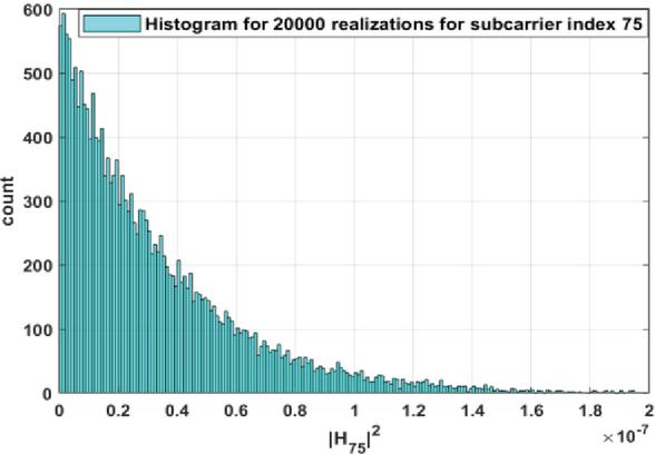
where with KHz, sub-channel bandwidth in 802.11ax, is the Boltzmann’s constant, and is the temperature in Kelvin. N is the total number sub-carriers in a bandwidth , is the channel gain at sub-carrier, is the total noise power, and is the total transmit power across bandwidth ‘B’. Considering the Rayleigh fading channel, the channel gain for each sub-carrier is exponentially distributed [12], as depicted in Figure 1a. Here, the subcarrier index is picked randomly. A histogram plot of 20,000 samples corresponding to 20,000 channel realizations follows the exponential distribution. We have . From Equation (1), with the total transmit power across 20 MHz operating bandwidth, .
IEEE 802.11ax supports OFDMA, where multiple subcarriers are grouped to form a resource unit (RU). Each RU is assigned to a user for data packet transmission. Since packets are the entities we transmit and receive, SNR per packet is a quantity of interest. The WLAN channel varies slowly; hence, the SNR is assumed to be static over the entire packet duration. The SNR for each packet is computed using the channel and noise estimates at the receiver. The channel estimates are obtained using the HE-LTF samples of the packet preamble transmitted over sub-carriers of the allotted RU. The average noise power is estimated using the pilot sub-carriers of the HE-data field. The SNR at the receiver over an RU of sub-carriers with ,
| (2) |
If sub-carrier SNRs, , are iid, since are exponentially distributed, the average SNR over sub-carriers of an RU (SNR per packet) is distributed according to a Gamma distribution [12, 13], Gamma (, ). is the number of sub-carriers in a RU, is the noise power, and is the parameter of the exponentially distributed channel gains at the sub-carrier.
We simulate a scenario of an Access Point (AP) transmitting to a user in a 20 MHz Bandwidth channel (OFDMA) at a carrier frequency of 5.25GHz using WLAN High Efficiency (HE) multi-user (MU) format packets as specified in IEEE 802.11ax [7].
Table 1
| Simulation parameters | |
| General Parameters | |
| Distance (d) | 12 m (NLOS) |
| Noise power (Pn) | 90 dBm |
| Transmit power per packet () | 1W |
| Packet size () | 500 bytes |
| Number of packets processed | 40,000 |
| Signal flow | Downlink |
| Target PER | 0.1 |
| Specific for IEEE 802.11ax | |
| Mode of transmission | OFDMA |
| RU allocation index | 192 |
| Number of RUs | 1 |
| Number of users | 1 |
| RU size () | 242 |
| Channel parameters | |
| Channel Bandwidth | 20 MHz |
| Carrier frequency | 5.25 GHz |
| Delay profile | Channel model-D |
| Environmental speed | 0.089 km/hr |
| Channel coding | LDPC |
| No. of penetration walls | 2 |
| Wall penetration loss | 2.5 dB |
| Pathloss | 74.62dB |
MATLAB WLAN Toolbox of MathWorks is used to model 802.11ax multi-user OFDMA downlink transmission over a TGax indoor fading channel. Table 1 summarizes the simulation parameters to evaluate our proposed rate adaptation algorithm, BLbRA, and HCDRA algorithm.
The RU allocation index property defines the number of RUs, the size of each RU, and the number of users assigned to each RU. The AP transmits a burst of 40,000 packets, and the client demodulates and decodes the packets. An evolving TGax indoor Rayleigh fading channel with AWGN is modeled between the AP and client device.
Figure 1a: Histogram of a channel gain at , .
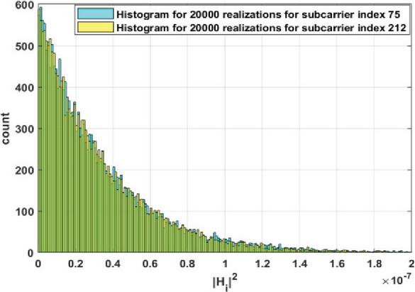
Figure 1b: Histogram overlap of and .
We mention some challenges faced during the experimentation, and the directions followed to overcome them.
• The initial plan was to use , the number of subcarriers in an RU, as the shape parameter () of the SNR probability distribution and learn the rate parameter ’R’ from the observed SNR measurements at the receiver. However, experiments showed that the learned distribution did not match the empirically observed SNR distribution. This resulted in overestimating the packet SNR, as shown in Figure 2.
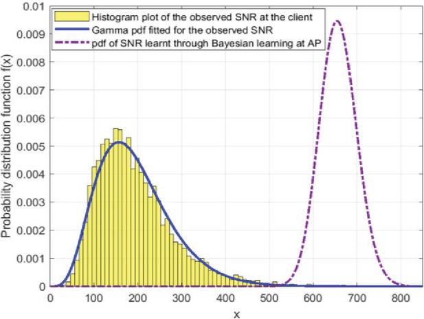
Figure 2 Histogram plot and Gamma pdf fit of the observed SNR at the client, SNR pdf learned through Bayesian learning by fixing the shape parameter, = 242.
• This observation made us suspect that the iid property among subcarriers could be assumed. We obtained the histogram plots of channel gains at sub-carrier indices , , as shown in Figure 1b. We further chose closely spaced sub-carrier indices to , to obtain their histogram plots and then concluded that the sub-carriers are identically distributed.
• To check the independence of channel gains over sub-carriers, we define two events for sub-carrier indices . Event falling in the interval (A1, B1)} and Event falling in the interval (A2, B2)}. Let N1 Number of occurrences of the joint event X AND Y, N2 Number of occurrences of event X, and N3 Number of occurrences of event Y, W width of an interval. We check for the probability condition for the two events X and Y to be independent, P (X and Y) P(X) P(Y). Table 2 summarizes the observed values.
Table 2
| Experimental data to check for the independence of channel gains at sub-carrier indices 75 and 212 | |||||||||
| (A1, B1) | (A2, B2) | W | N1 | N2 | N3 | P (X AND Y) | P(X) | P(Y) | P(X) P(Y) |
| [0.2e-7, 0.21e-7] | [0.6e-7, 0.61e-7] | 0.01e-7 | 3 | 339 | 107 | 1.50e-04 | 0.01695 | 0.00535 | 0.9069e-04 |
| [0.2e-7, 0.22e-7] | [0.6e-7, 0.62e-7] | 0.02e-7 | 7 | 656 | 202 | 3.50e-04 | 0.03280 | 0.01010 | 3.3128e-04 |
| [0.2e-7, 0.23e-7] | [0.6e-7, 0.63e-7] | 0.03e-7 | 11 | 967 | 304 | 5.50e-04 | 0.04835 | 0.01520 | 7.3492e-04 |
| [0.2e-7, 0.24e-7] | [0.6e-7, 0.64e-7] | 0.04e-7 | 19 | 1273 | 386 | 9.50e-04 | 0.06365 | 0.01930 | 12.2845e-04 |
• The experimentation suggested that subcarrier SNRs, are not independent. This is because the channel gains at any two sub-carriers are not independent. The channel gains of sub-carriers are significantly correlated due to the channel coherence bandwidth. Therefore, multipath propagation has an impact on the channel gain or SNR statistics.
However, we found the empirical distribution of observed packet SNR at the receiver to match the Gamma distribution closely, as shown in Figure 2. Then, we wondered if the Gamma distribution could be ”tuned” to match observed histograms by adjusting its parameters. Ideally, both parameters should be learned. However, the literature indicates that learning both parameters is hard. The conjugate prior for the Gamma rate parameter is known to be Gamma distributed, but no standard distribution behaves as the prior for the shape parameter [14]. So, we decided to keep the shape parameter, , fixed and learn the rate parameter (R) through Bayesian learning.
The next question that arose was, what value to be chosen for . We use the range of desirable SNR from past channel measurements as a piece of prior information to choose the shape parameter’s value. We had two criteria: (i) we wanted the SNR pdf to cover the full range of possible SNR values from 0 to 28dB, modeling all possible channel conditions. (ii) we wanted the shape of the pdf not to become symmetric around its mean value. We did some experiments to study the effect of the shape parameter, , on the gamma pdf by fixing the scale parameter , 20, 30, 40 and 50. The pdf spread is smaller than the desired range for lower values of , up to 5. For larger values of beyond 7, the mean of the distribution shifts towards the right, and the support of the distribution does not include lower values of observed SNR. Also, higher values of , beyond 15, resulted in a more concentrated distribution around its mean. So, we prefer to choose and estimate R (1/) through Bayesian learning. This method yielded an excellent match with the experimentally observed receiver SNR histogram and the gamma distribution learned by Bayesian learning.
Bayesian Learning (BL) of the Rate Parameter of the Gamma Distribution To find the posterior probability of the Gamma distributed rate parameter R, we use the Bayes rule,
| (3) |
where is a positive vector of observed SNR per packet. Since the denominator only depends on observed data, the posterior is proportional to the likelihood multiplied by the prior
| (4) |
Obtaining analytical solutions for the rate parameter R requires using conjugate priors. A prior is called conjugate with a likelihood function if the prior functional form remains unchanged after multiplication by the likelihood distribution [14]. A well-known conjugate prior for the rate parameter R of the Gamma distribution is a Gamma distribution parameterized using shape d and rate e,
| (5) |
Given the observation vector , and multiplying its Gamma likelihood by the prior on the rate (5), we get its posterior [14], with
| (6) |
where is the shape parameter of the Gamma likelihood distribution of the SNR per packet (), is the measured SNR of the packet, and n is the number of SNR observations. We call ‘n’ as the rate parameter update window.
Let the SNR probability density function (pdf) at the transmission time be denoted by . The initial rate parameter, , is chosen based on past measurements from the expectation of the likelihood distribution of average SNR, . Initially, we generate an SNR sample using SNR pdf . Though several sampling techniques exist [10], we describe one such technique called inverse CDF sampling. It is computationally efficient and easily implementable.
• First, the cumulative distribution function (CDF) is calculated using (7).
| (7) |
• Generate a uniformly distributed random variable, .
• Finally, map to an SNR sample through the inverse SNR CDF, , where is the SNR sample or the SNR point estimate at the transmission instant, and .
The sampling of the updated SNR pdf is done for every packet transmission, so the MCS is selected based on the sampled SNR. The selected MCS is used for the next packet transmission. The client device measures the SNR per packet using the channel and noise estimates and computes the sum of the measured average SNR for ‘n’ packets. The sum, is fed back to the AP using the standards-compliant HE-CQI report field. The rate parameter R’s hyperparameters are updated using (6) after every ‘n’ packets (rate parameter update window). The posterior expectation of the rate parameter is calculated using the recently updated (, ) pair. The updated value of is further used to update the pdf of the average SNR gamma (6, ).
The Bayesian update channel SNR model simulation is done using the standards-compliant, credible link simulator MATLAB WLAN Toolbox of MathWorks. Fixing the shape parameter, to 6, and learning the rate parameter, R, through Bayesian learning resulted in an excellent match with the experimentally observed receiver SNR histogram at the client and the SNR pdf learned through Bayesian learning at AP.
The pdf of SNR iteratively concentrates around the true channel SNR, i.e., assigns a higher probability density to the SNRs close to the true channel SNR. This is depicted in Figure 3a. Figure 3b shows the perfect overlap of the CDF of the observed SNR at the client and the CDF learned at AP through Bayesian learning.
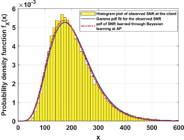
Figure 3a: Histogram plot and Gamma pdf fit of the observed SNR at the client, and SNR pdf learned through Bayesian learning by fixing .
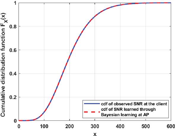
Figure 3b: CDF of observed SNR and Learned SNR.
The posterior SNR pdf learned through Bayesian learning is sampled for every packet transmission to get the SNR sample or the SNR point estimate. The SNR sample is mapped to the PER for all MCS (0–9) through a fast Received Bit Information Rate (RBIR) based offline link PLA model table lookup [15, 16, 17]. RBIR is described in detail in our previous work [15]. We select the highest MCS for which the estimated PER target PER (0.01).
For every successful packet transmission, there is some link margin. It is the difference between the instantaneous channel SNR (actual) and the minimum SNR (dependent on MCS) required for the successful decoding of the packet [18]. BLbRA addresses link margin by choosing the MCS for every packet transmission. BLbRA has lower computational complexity for computing the optimal MCS using RBIR table lookup and requires lower memory to store the SNR model. In our algorithm, the Access Point (AP) performs the Bayesian learning of the rate parameter of the SNR and decides the optimal MCS, taking off the computational load from the client device.
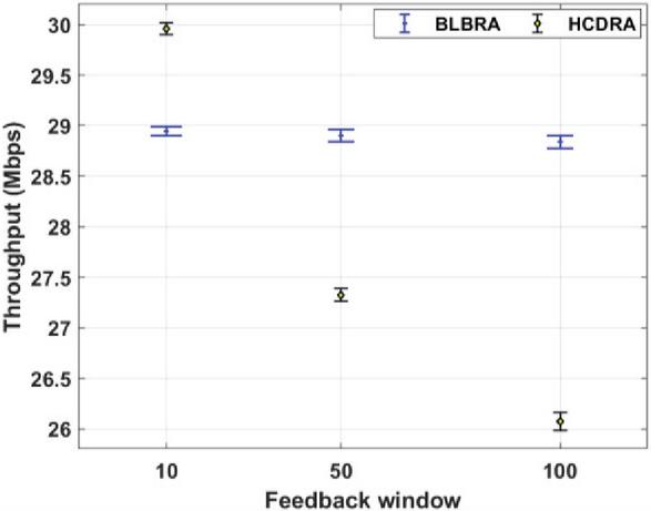
Figure 4a: Throughput (Mbps) with 95% confidence level.
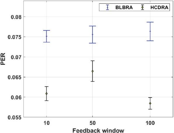
Figure 4b: PER with 95% confidence level
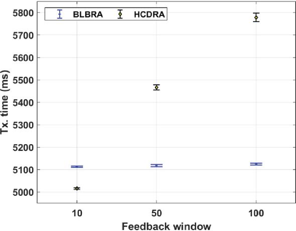
Figure 4c: Transmission time (ms) with 95% confidence level with increasing feedback window.
This section presents the throughput comparison of BLbRA and Hybrid Channel-Dependent Rate Adaptation (HCDRA), an algorithm we proposed earlier in [15]. Figures 4a, 4b and 4c show the throughput, PER and transmission time of both algorithms. For each presented results, we show the mean value over the 20 simulation runs with 95% confidence level.
HCDRA performs rate adaptation based on fresh channel estimates for every SNR feedback window. The per-RU average SNR derived from the channel estimates is fed back through HE Channel Quality Indicator (CQI) report field. The SNR feedback window (FBW) is set to 10, 50, and 100 packets. We observed that the throughput decreases in HCDRA as the FBW increases. This is because HCDRA uses the same MCS for all the packets transmitted for every SNR feedback window unless the probe packet fails or if two consecutive packets fail within the FBW (refer to Step. 5a of [15]).
In BLbRA, the rate parameter update window ‘n’ (of Equation (6)) is set to 10, 50, and 100 packets to compare the throughput performance with HCDRA. Here the sum of per-RU average SNR for ‘n’ packets is fed back to the AP using the standards-compliant HE-CQI report field. With the rate parameter update window of n 10 packets, BLbRA throughput performance is close to HCDRA with FBW of 10 packets. However, we observed that throughput and PER performance of BLbRA with increased rate parameter update window of n 50 and n 100 remains on par with n 10 packets.
HCDRA has a lower PER than BLbRA. This is because HCDRA becomes very conservative as feedback window increases compromising on the throughput gain. Unlike HCDRA, the transmission time in BLbRA is consistently smaller for n 50 and 100, emphasizing the fact that BLbRA chooses a higher MCS for most of the packet transmissions.
Figure 5 shows the histogram plot of MCS used in BLbRA and HCDRA for a feedback window of 100. It is evident that the BLbRA uses higher order MCS larger compared to HCDRA, leading to a throughput gain.
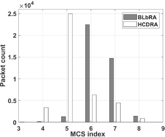
Figure 5 Histogram of the MCS used in BLbRA (n=100) and HCDRA (FBW=100).
Table 3
| Performance of BLbRA (n 100) within the window of N/4 packets | ||||
| Packet | 1 to | N/4 to | N/2 to | 3N/4 |
| Number | N/4 | N/2 | 3N/4 | to N |
| Throughput (Mbps) | 28.7458 | 28.8675 | 28.8256 | 28.7661 |
| PER | 0.0775 | 0.0769 | 0.0773 | 0.0761 |
| Transmission time (ms) | 1282.32 | 1280.31 | 1281.49 | 1282.47 |
Table 3 shows the performance metric for BLbRA (n 100) within the transmission window of N/4 packets, with N 40K packets. The throughput and PER are consistent within each transmission window. This is because the MCS in BLbRA is obtained by mapping the SNR point estimate for every packet transmission, as explained in section 3D. The BLbRA addresses the link margin for every packet transmission, thus transmitting the higher-order MCS whenever the channel supports it.
We designed the Bayesian Learning based rate adaptation to decide on the MCS for the next packet by sampling the learned SNR distribution at the AP and pretending that the sampled value is the SNR that the next packet will see. To evaluate both algorithms, we modeled the end-to-end link-level SISO transmit-receive link with IEEE standard-defined channel models [7, 16]. BLbRA learns from the observed SNR feedback (after every rate parameter update window) to obtain the SNR estimate; the estimates closely match the true channel SNR. The rate parameter update window is increased to see the effect on throughput. BLbRA continues to perform well even with the reduced feedback overhead.
BLbRA is eminently implementable using the feedback mechanism recommended by the IEEE 802.11ax standard. Therefore, no customized mechanisms are needed to implement our proposed algorithm. Further, we would like to extend Bayesian learning to explore the possibility of learning both the parameters of Gamma distributed SNR and evaluate the throughput and PER performance of the link adaptation algorithm.
Sheela C S is supported by a fellowship grant from the Centre for Networked Intelligence (a Cisco CSR initiative) of the Indian Institute of Science, Bangalore, India.
[1] A. Kameman and L. Montban, “WaveLAN II: A high-performance wireless LAN for the unlicensed band,” Bell Labs Technical Journal, pp. 118–133, 1997.
[2] M. Lacage, M. H. Manshaei, and T. Turletti, “IEEE 802.11 rate adaptation: a practical approach,” Proceedings of the 7th ACM international symposium on Modelling, analysis, and simulation of wireless and mobile systems, pp. 126–134, 2004.
[3] Dong Xia, Jonathan Hart, Qiang Fu, “On the Performance of Rate Control Algorithm Minstrel,” IEEE 23rd International Symposium on Personal, Indoor, and Mobile Radio Communications – (PIMRC), 2012.
[4] M. Vutukuru, H. Balakrishnan, and K. Jamieson, “Cross-layer wireless bit rate adaptation,” ACM SIGCOMM 2009, Vol. 39, Issue 4, 2009.
[5] S. Khan, S. A. Mahmud, H. Noureddine, H. S. Al-Raweshidy, “Rate-adaptation for multi-rate IEEE 802.11 WLANs using mutual feedback between transmitter and receiver,” IEEE 21st International Symposium on Personal Indoor and Mobile Radio Communications, 2010.
[6] J. Zhang, K. Tan, J. Zhao, H. Wu, and Y. Zhang, “A practical SNR guided rate adaptation,” IEEE International Conference on Computer Communications (INFOCOM), Phoenix, AZ, USA, 2018.
[7] “IEEE P802.11ax/D4.1 Draft Standard for Information technology – Telecommunications and information exchange between systems Local and metropolitan area networks – Specific requirements – Part 11: Wireless LAN Medium Access Control (MAC) and Physical Layer (PHY) Specifications,” IEEE P802.11ax/D4.1, April 2019.
[8] Saman Atapattu, Chintha Tellambura, and Hai Jiang, “A mixture gamma distribution to model the SNR of wireless channels”, IEEE transactions on wireless communications 10.12 (2011), pp. 4193–4203.
[9] P Mohana Shankar. Fading and shadowing in wireless systems. Springer, 2017.
[10] Vidit Saxena , Hugo Tullberg, and Joakim Jaldén, “Reinforcement Learning for Efficient and Tuning-Free Link Adaptation”, IEEE Transactions on Wireless Communications, Vol. 21, No. 2, February 2022.
[11] R. Patidar, S. Roy, T. Henderson, and A. Chandramohan, “Link-to-System Mapping for ns-3 Wi-Fi OFDM Error Models,” Workshop on ns-3, June 2017.
[12] Andrea Goldsmith, “Wireless Communications”, Cambridge University Press, 2005.
[13] Ross, Sheldon M, “Introduction to probability and statistics for engineers and scientists”, 4th edition, 2009.
[14] A. Llera, C. F. Beckmann, “Bayesian estimators of the Gamma distribution”, Technical report by Radboud University Nijmegen and Donders Institute for Brain Cognition and Behaviour, July 2016.
[15] Sheela C S, Joy Kuri, Nadeem Akhtar, “Performance Analysis of Channel-Dependent Rate Adaptation for OFDMA transmission in IEEE 802.11ax WLANs”, Workshop on Standards-driven Research, COMSNETS, Jan. 8, 2022.
[16] R. Porat, Matt Fischer, IEEE 802.11-14/0571r12, “IEEE P802.11 Wireless LANs: 11ax Evaluation Methodology,” Jan 2016.
[17] K. Brueninghaus, D. Astely, T. Salzer, S. Visuri, A. Alexiou, S. Karger, and G. Seraji, “Link performance models for system-level simulations of broadband radio access systems,” in IEEE 16th International Symposium on Personal, Indoor and Mobile Radio Communications. IEEE, 2005.
[18] A. Cidon, K. Nagaraj, S. Katti, and P. Viswanath, “Flashback: Decoupled lightweight wireless control,” in Proc. ACM SIGCOMM, Vol. 42, Issue 4, Oct. 2012, pp. 223–234.
[19] I. Sammour and G.Chalhoub, “Evaluation of Rate Adaptation Algorithms in IEEE 802.11 Networks,” Electronics 2020, No. 9, 1436, Sept 2020.
[20] Pengfei Xia, Ron Murias, IEEE 802.11-14/0527-r1, “PHY Layer Abstractions for TGax System Level Simulations,” May 2014.

Sheela C S (Student Member, IEEE) is a Ph.D. student in the Department of Electronic Systems Engineering, Indian Institute of Science, Bangalore, India. She received M. Tech. degree from the department of Electronics and Electrical Communication Engineering, Indian Institute of Technology Kharagpur in 2012. Before joining IISc for the Ph.D. program, she worked as an Assistant Professor at R. V. College of Engineering, Bangalore during 2012–18. Her research interests include PHY Layer signal processing, channel modeling, machine learning for wireless communication and wireless communication systems building using MATLAB toolboxes. She is currently working on Learning based rate adaptation techniques for the next-generation IEEE WLAN standard.

Joy Kuri is a Professor in the Department of Electronic Systems Engineering, Indian Institute of Science (IISc), Bangalore, India. He has a M.E. from the Department of Electrical Communication Engineering at the IISc. He went on to receive a PhD from the same department at IISc in 1995. Subsequently, he spent two years at Ecole Polytechnique, University of Montreal, Canada and one and a half years in INRS-Telecommunications, University of Quebec, Canada as a Research Associate. Since 1999 he has been with the Department of Electronic Systems Engineering, IISc.
He is the coauthor of two widely cited books and has authored or coauthored 120 articles in peer-reviewed journals and conferences. Over the last two decades, his research and teaching interests included stochastic modelling, analysis, design and control of networks arising in various application contexts, including communication, information dissemination, security, transportation, and power. During June 2014–July 2016, he was an Associate Editor for the IEEE/ACM Transactions on Networking.